Exploring the field

Satellite photogrammetry in a nutshell

As its name suggests, satellite photogrammetry works using optical satellite acquisitions to generate a Digital Surface Model, the 2.5D representation created from observed surface altitude data. We speak of 2.5D because the digital surface model is an array of pixels (raster, 2D) where each pixel (x,y) corresponds to an altitude (z).

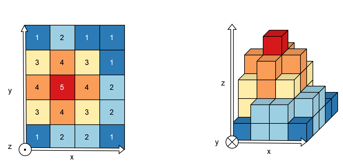
Fig. 1 2.5D representation

On the left, an example of an array of pixels, and on the right, a volume representation of altitude values.

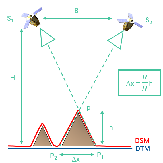
Like our eyes, altitude (or depth relative to the satellite, to continue the analogy) is determined from the observed pixels displacement. We therefore need at least two images, acquired from two different viewpoints. This difference in viewpoint between two satellites is quantified by the B over H ratio where B is the distance between the two satellites and H is their altitude.

B over H ratio	Two viewpoints

Every raster GDAL knows how to read can be given as CARS input. In addition to images, the photogrammetric process requires geometric models. Rational Polynomial Coefficients (RPCs) provide a compact representation of a ground-to-image geometry giving a relationship between:

• Image coordinates + altitude and ground coordinates (direct model: image to ground)

• Ground coordinates + altitude and image coordinates (inverse model: ground to image)

These coefficients are classically contained in the RPC*XML files.

From Satellite Images to Digital Surface Model

Generate a DSM step by step

Images are first resampled in epipolar geometry: by changing viewpoints, objects pixels move along a line.

This enables a one-dimensional search (computer performance + error limitation).

The pixels shifting along others directions doesn’t taking account and it corresponds to fast moving objets (for instance like vehicle moving from bottom to top, see below)

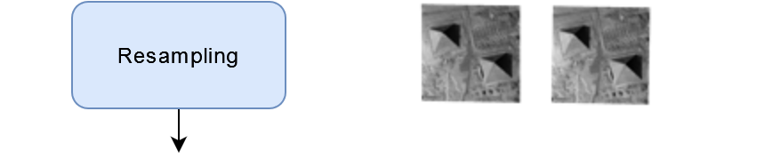
Pipeline	Resampling

For each point in one image, the software searches the corresponding point in the other image.

The color of the pixels (grayscale) in the image below corresponds to the shift value. Some pixels do not have a match (matching error due to moving objects, shadows etc.).

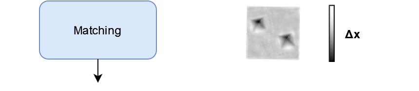
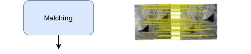
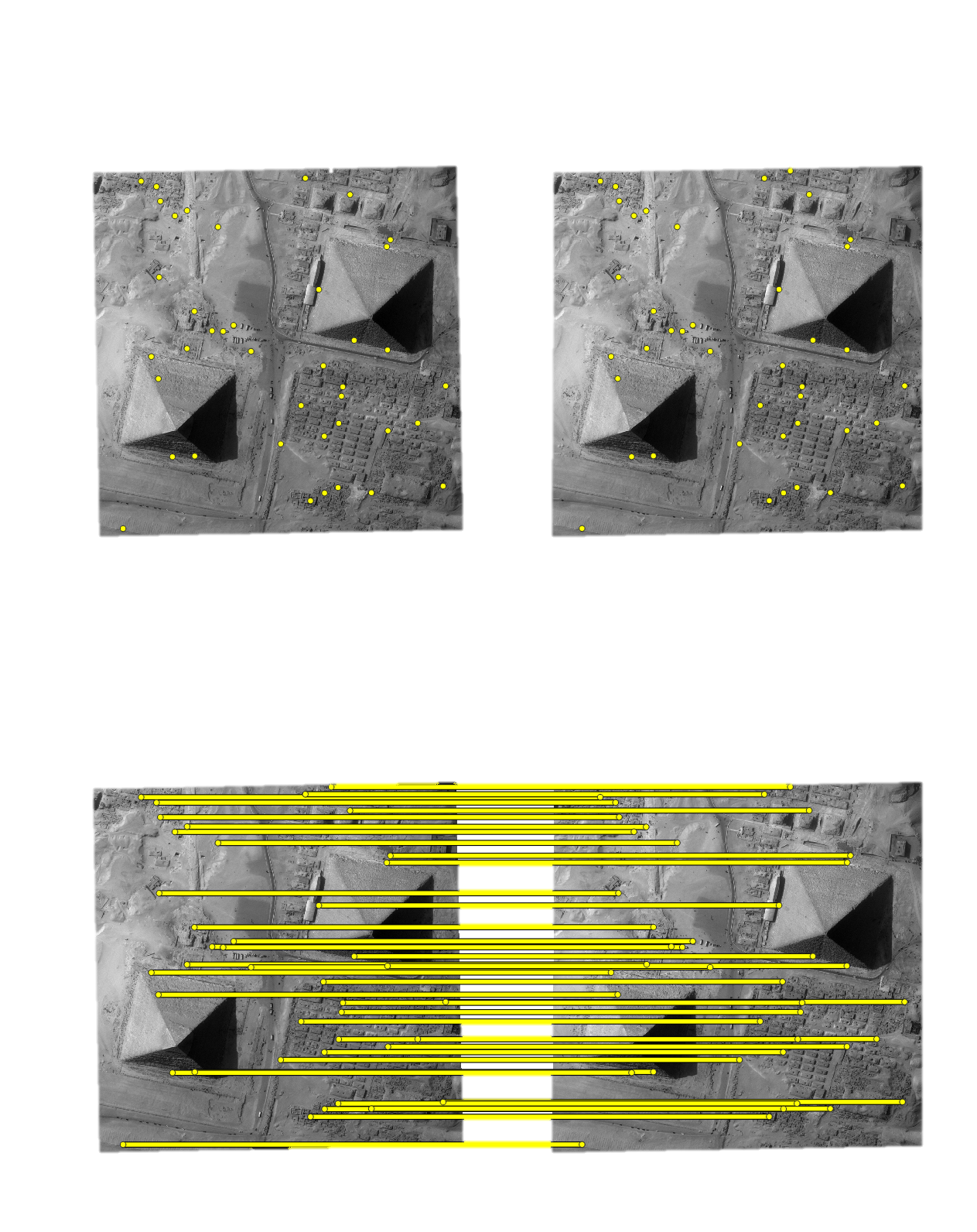
Pipeline	Matching

The displacements obtained are transformed into positions in both images.

This allows to deduce lines of sight. The intersection of these lines gives a point in space: longitude, latitude, altitude (see below).

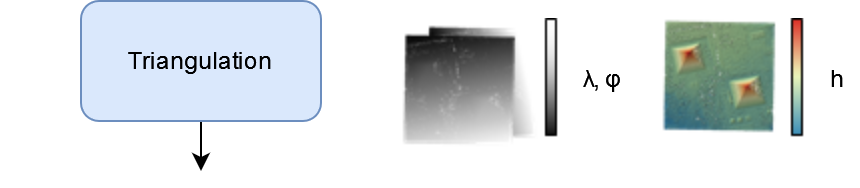
Pipeline	Triangulation

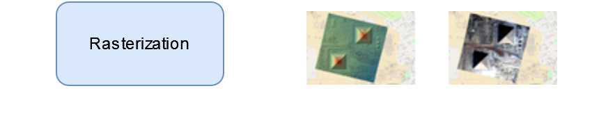
To obtain a raster image, the final process projects each point into a 2D grid: altitudes and colors (see below).

Pipeline	Rasterization

Initial Input Digital Elevation Model

For now, CARS uses an initial input Digital Elevation Model (DEM) which is integrated in the stereo-rectification to minimize the disparity intervals to explore. Any geotiff file can be used.

For example, the SRTM data corresponding to the processed zone can be used through otbcli_DownloadSRTMTiles.

The parameter is initial_elevation as seen in Configuration.

Altimetric exploration and geometric inaccuracies

To reduce the search interval (i.e. altimetric exploration) in the matching step and thus save computing time, a faster sparse matching step is typically used. This matching step also enables geometric errors to be corrected, thus ensuring that the epipolar geometry (based on these models) is correct.

Matching can be performed with keypoints like SIFT.

Pipeline	Matching (sparse)

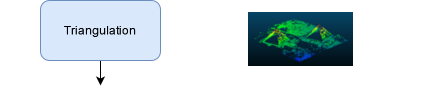
The result is a sparse point cloud…

Pipeline	Triangulation (sparse)

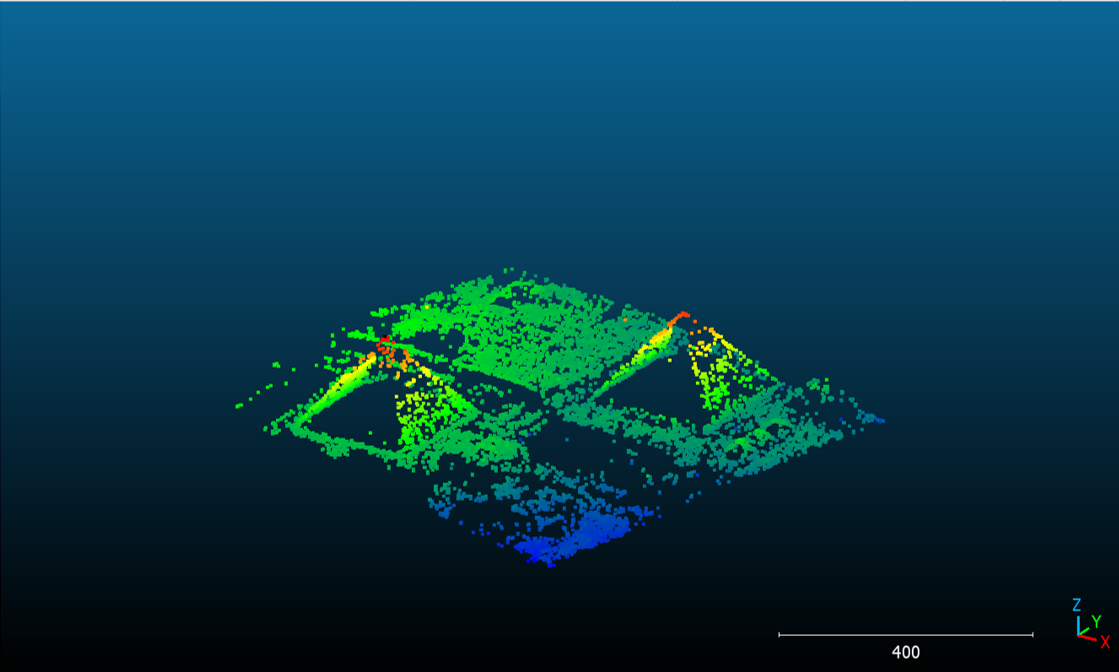
and a sparse digital surface model.

Pipeline	Rasterization (sparse)

Mask and Classification Usage

Photogrammetry is a technique that cannot reproduce altitude on water. This technique also has difficulties for moving elements or in shaded areas.

For this reason, it is possible to mask out areas or apply ad hoc processing to aid the matching stage.

Masks

CARS can use a mask for each image in order to ignore some image regions (for instance water mask). This mask is taken into account during the whole 3D restitution process.

The masks have one band with 1 nbit and the non zeros values will be considered as invalid data and theses areas will not processed during the computation.

Please, see the section Convert image to binary image to make a binary image.

The mask are resampled in epipolar geometry with the resampling application.

The masked values are not taken into account in the matching process (sparse or dense matching method) to avoid mismatch and useless processing.

Further, the sparse matching estimation of the disparity range can be enhanced with mask using for the water area typicaly.

Classification

The considered classification image are multi-band raster with descriptions name for each band and 1 nbit per band. See optional description option of the Gdal band raster model

Please, see the section Convert image to binary image to make a multiband binary image with 1 bit per band.

All non-zeros values of the classification image will be considered as invalid data.

The classification can be used in each application by band name list selection parameter. See application classification parameter Configuration..

3D products

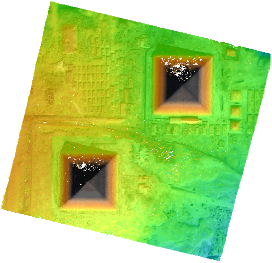
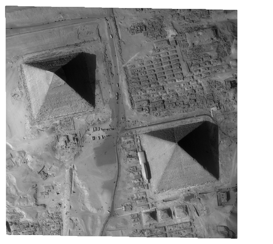
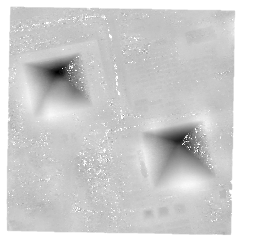
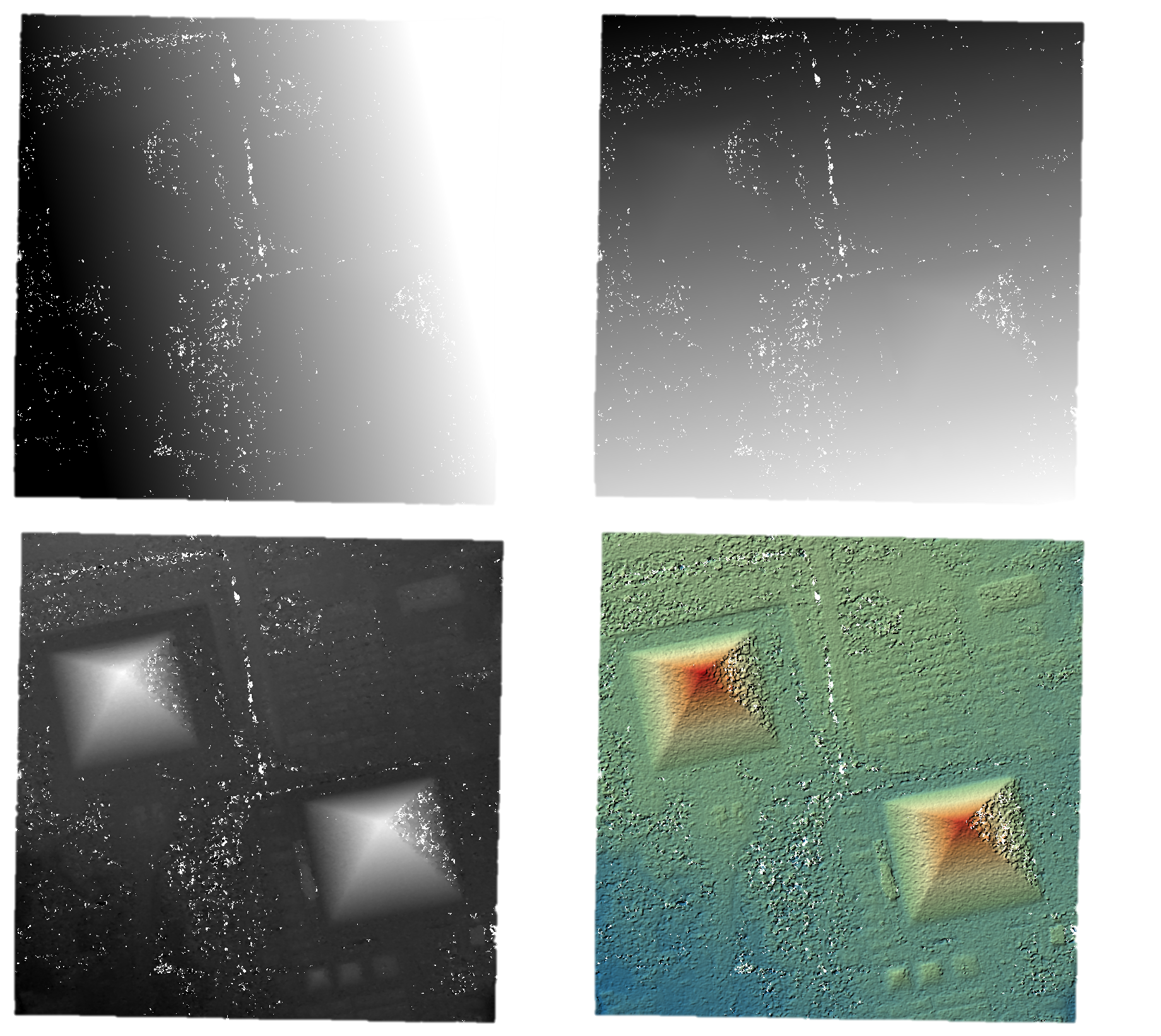
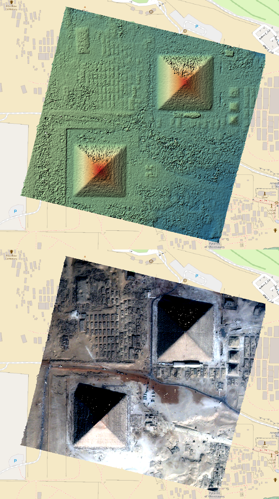
CARS produces a geotiff file named dsm.tif that contains the Digital Surface Model in the required cartographic projection and the ground sampling distance defined by the user.

If the user provides an additional input image, an ortho-image clr.tif is also produced. The latter is stackable to the DSM (See Getting Started).

If the user saves points clouds as laz format (point_cloud_fusion, point_cloud_outliers_removing, point_cloud_rasterization), the points clouds are saved in laz compressed format with colors or graylevel image.

These two products can be visualized with QGIS for example.

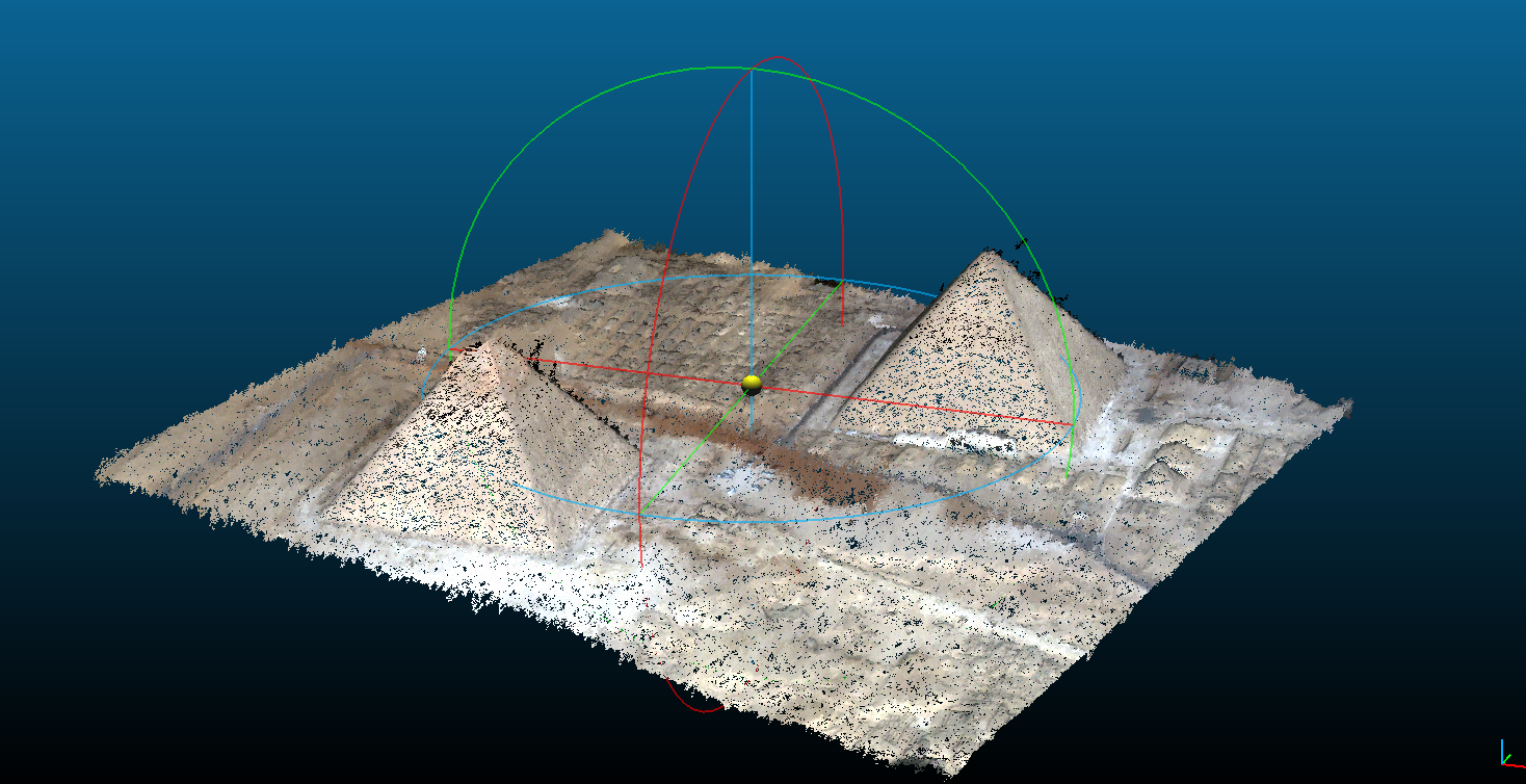
dsm.tif	clr.tif	QGIS Mix	cloudcompare