Technical Foundations

Satellite photogrammetry in a nutshell

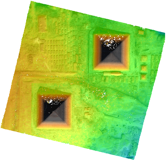
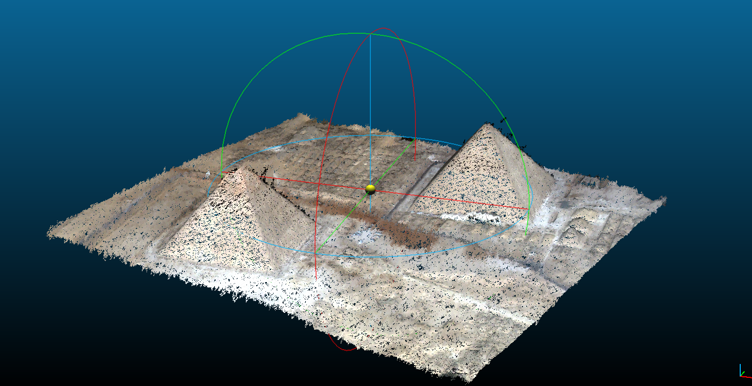
As its name suggests, satellite photogrammetry works using optical satellite acquisitions to generate a Digital Surface Model (DSM), the 2.5D representation created from observed surface altitude data. We speak of 2.5D because the digital surface model is an array of pixels (raster, 2D) where each pixel (x,y) corresponds to an altitude (z).

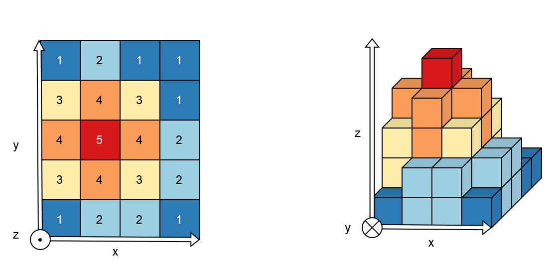
Fig. 1 2.5D representation

On the left, an example of an array of pixels, and on the right, a volume representation of altitude values.

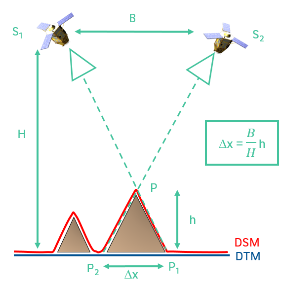
Like our eyes, altitude (or depth relative to the satellite, to continue the analogy) is determined from the observed pixels displacement. We therefore need at least two images, acquired from two different viewpoints. This difference in viewpoints between two satellites is quantified by the B over H ratio where B is the distance between the two satellites and H is their altitude.

B over H ratio	Two viewpoints

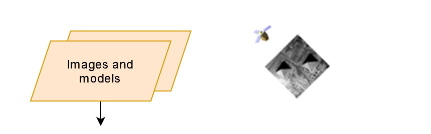
Every raster readable by GDAL can be given as CARS input. In addition to images, the photogrammetric process requires geometric models. Rational Polynomial Coefficients (RPC) provide a compact representation of a ground-to-image geometry giving a relationship between:

• Image coordinates + altitude and ground coordinates (direct model: image to ground)

• Ground coordinates + altitude and image coordinates (inverse model: ground to image)

These coefficients are classically contained in the RPC*.XML files.

From Satellite Images to Digital Surface Model

Generate a DSM step by step

Images are first resampled in epipolar geometry: by changing viewpoints, objects pixels move along a line.

This enables a one-dimensional search (computer performance + error limitation).

The pixels shifting along other directions are not taken into account : it corresponds to fast moving objects like vehicles.

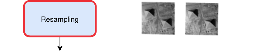
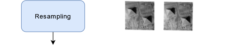
Pipeline	Resampling

For each point in one image, the software searches the corresponding point in the other image.

The color of the pixels (grayscale) in the image below corresponds to the shift value. Pixels with no match are displayed as transparent pixels in the image below.

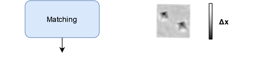
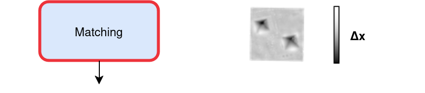
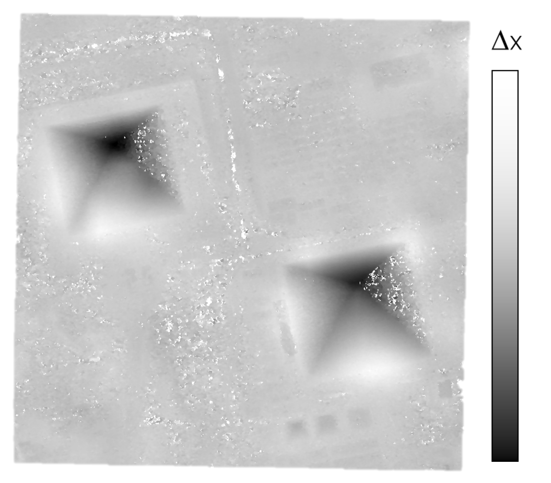
The transparent pixels indicate areas where the matching algorithm couldn’t find a reliable correspondence between the two images, highlighting regions of uncertainty in the matching process. These matching errors can occur due to various reasons such as moving objects, shadows, occlusions, or areas with insufficient texture.

Pipeline	Matching

The displacements obtained are transformed into positions in both images.

This allows to deduce lines of sight. The intersection of these lines gives a point in space: longitude, latitude, altitude (see below).

A line of sight is an imaginary straight line from the camera’s perspective through a specific point in the image, extending into 3D space. It represents all possible 3D positions that could have produced that image point.

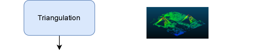
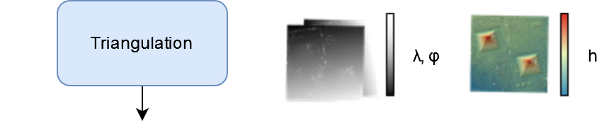
Pipeline	Triangulation

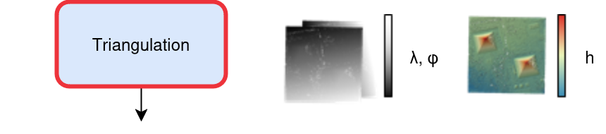
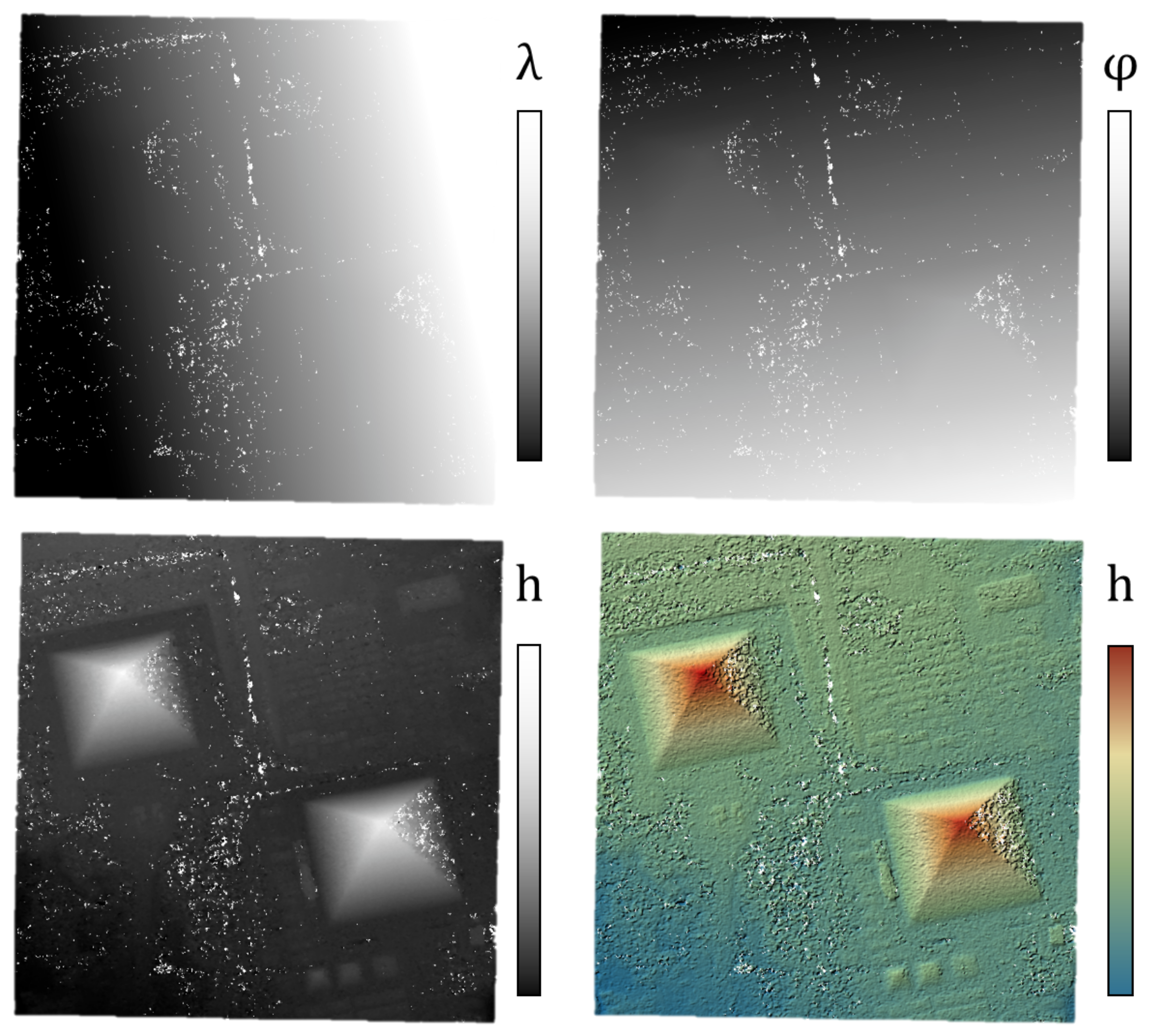
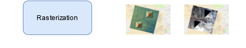
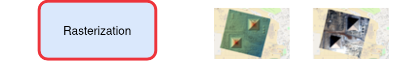
To obtain a raster image, the final process projects each point into a 2D grid: altitudes and colors (see below).

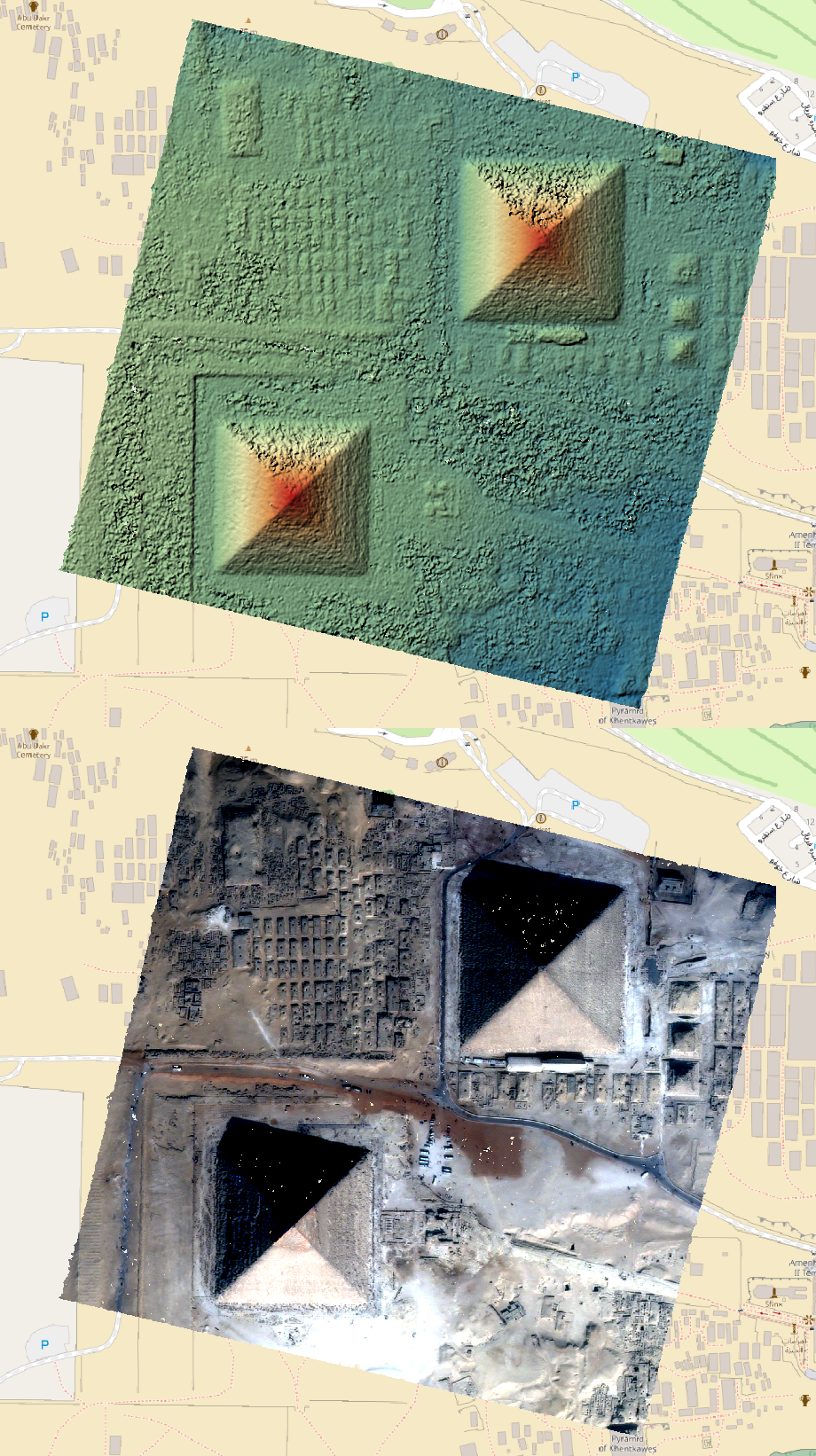
Pipeline	Rasterization

Altimetric exploration at multiple resolutions

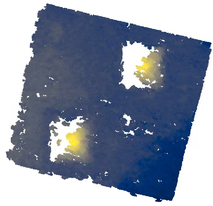
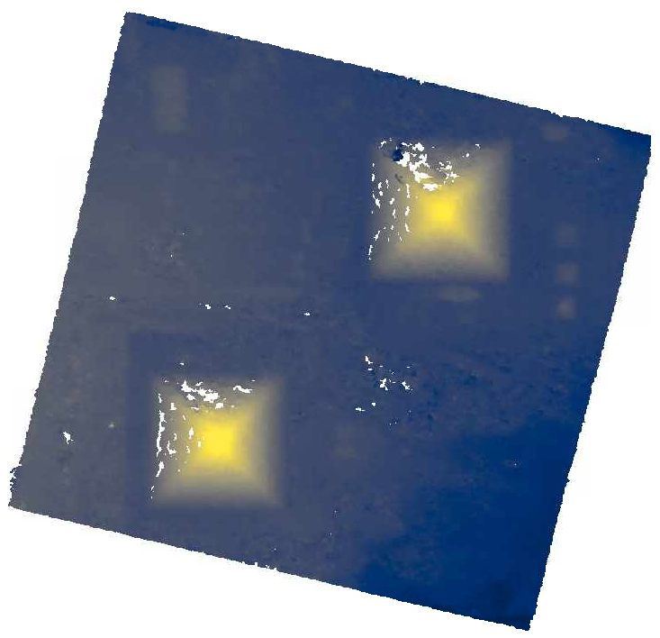
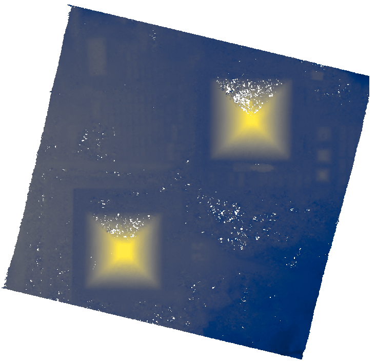
To reduce the search interval (i.e. altimetric exploration) in the dense matching step and thus save computing time, CARS’s pipeline runs the dense matching algorithm and surrounding applications at multiple resolutions, going from a very low resolution to the highest. Each time, based on the previous resolution, the disparity interval searched will be reduced.

This reduces computation time greatly while providing better results than a bruteforce approach.

DSM at resolution 4	DSM at resolution 2	DSM at resolution 1

With :

• resolution 4 corresponding to 4 times the original resolution (e.g., 4m if the original resolution is 1m).

• Resolution 2 corresponding to 2 times the original resolution (e.g., 2m if the original resolution is 1m).

• Resolution 1 corresponding to the original resolution (e.g., 1m).

Geometric inaccuracies

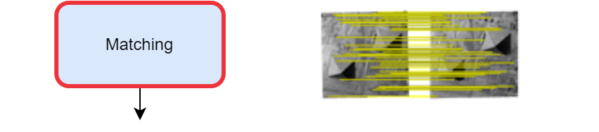
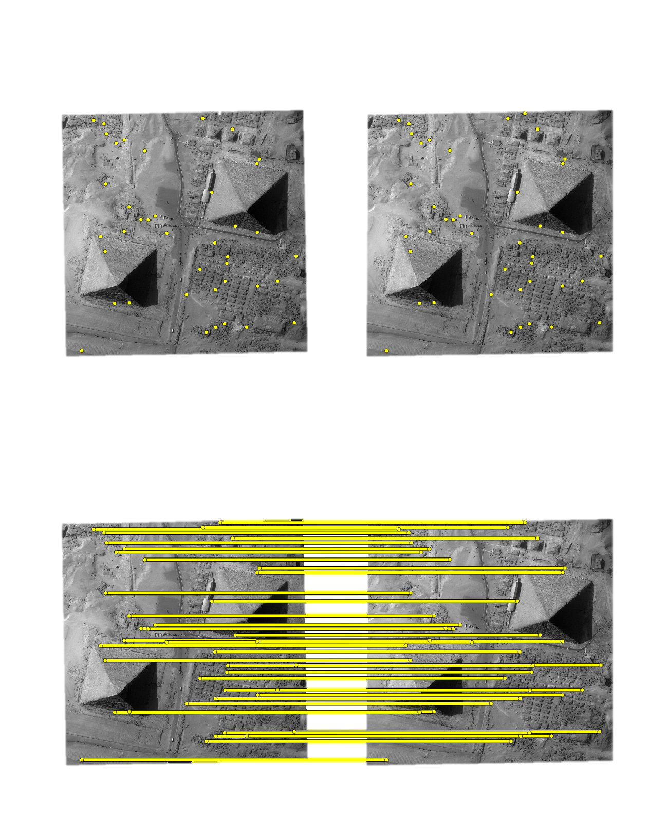
To reduce geometric errors present in the sensor images’ geometry model, a sparse matching step is performed on the full-resolution images in 2D. These matches are then used to correct geometric errors in the geometry model, ensuring that the epipolar geometry is correct, in turn allowing for better results.

Those matches will also be used to reduce the disparity interval searched in the pipeline’s first resolution run.

This sparse matching step is performed with keypoints, like SIFT to ensure that the matches found are accurate, as inaccurate ones may result in distortions and bad dense matching results. (SIFT Article:).

Pipeline	Matching (sparse)

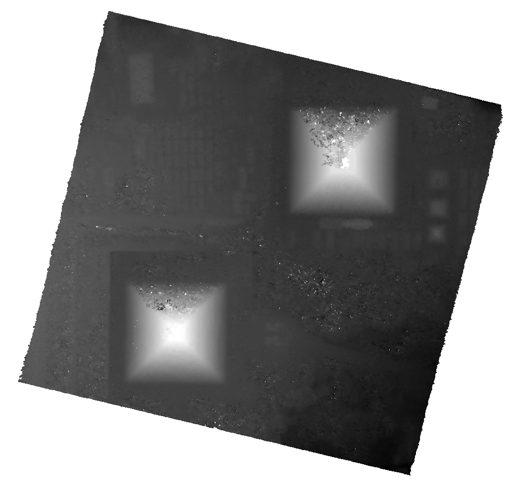
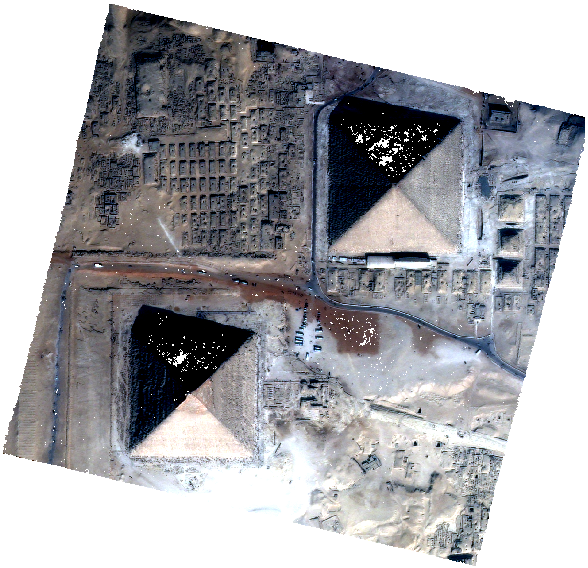
3D products

CARS produces a geotiff file named dsm.tif that contains the Digital Surface Model in the required cartographic projection and the ground sampling distance defined by the user.

An ortho-image image.tif is also produced from the first (left) sensor image of each pair. The latter is stackable to the DSM (See Quick start).

If the user saves point clouds as laz format, the point clouds are saved in laz compressed format with colors or graylevel image.

These two products can be visualized with QGIS for example.

dsm.tif	image.tif	QGIS Mix	cloudcompare

Pipeline overview

To summarize, CARS’s default pipeline is organized into sequential steps, starting from input pairs (and metadata) and producing output data. Each step is performed tile-wise and distributed among workers. Part of the pipeline operates at multiple spatial resolutions to reach the final results while minimizing computation time. It is possible to run CARS at a single resolution, but this may be very inefficient for large or medium size images.

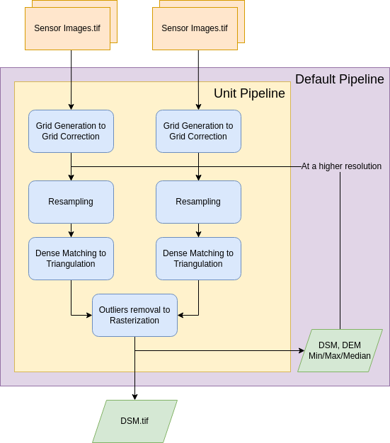
The pipeline will perform the following steps [Michel J. et al, 2020] [Youssefi D. et al, 2020]:

• For each stereo pair:

  1. Create stereo-rectification grids for left and right views.

  2. Resample both images into epipolar geometry.

  3. Compute sift matches between left and right views in epipolar geometry.

  4. Create a bilinear correction model of the right image’s stereo-rectification grid in order to minimize the epipolar error. Apply the estimated correction to the right grid.

• For each resolution (first_resolution, intermediate_resolution, last_resolution)

  • For each stereo pair:

    5. Resample the stereo pair in epipolar geometry, at the specified resolution using:

       • The input DTM (such as an SRTM) for the first resolution.

       • The DEM Median from the previous resolution for intermediate_resolution or last_resolution.

    6. Compute the disparity map in epipolar geometry, by using the DEM Min and DEM Max as disparity intervals. For the first resolution, sift features are used to refine the disparity intervals.

    7. Triangulate the matches and get for each pixel of the reference image a latitude, longitude and altitude coordinate.

  • Then

    8. Merge points clouds coming from each stereo pairs.

    9. Filter the resulting 3D points cloud via two consecutive filters: the first removes the small groups of 3D points, the second filters the points which have the most scattered neighbors.

    10. Rasterize: Project these altitudes on a regular grid to create a DSM and its associated color, as well as (if not at the last resolution) DEM Min/Max/Median.